Data Preparation and Cleaning

In this section, you will prepare and clean relevant datasets needed for task 2.

The main overview that is needed for Task 2 are as follows:

• Data processing
• Computation of the criteria
• Calculating the normalised distance
• Assessing the site suitability.

Data Processing

• In this section, we will go through how to get the data in an appropriate form which we can use to calculate the normalised distance. We will get all the data here into a raster format for the next step under “Calculating Normalised Distance”.
• There are several criteria to be used:
  • Distance from river/coastline/natural disasters: We use the river layer (flooding) because there are no other avoidable natural disasters. Follow section 2.1.
  • Slope: We use the slope layer generated from the DEM that was used for task 1, which is already rasterised. Hence no extra work to be done for this layer in this section.
  • Distance from Airport: We use both vector layers that had been used to create the overlay maps for task 1, but buffered. Follow section 2.3.
  • Distance from Urban Settlement: We use the Urban Settlements vector layer, clipped against the city boundaries. Follow section 2.4.
  • Distance from Forest Fire: We use the forest fire heatmap layer that had been created in task 1.
  • Distance from Road and Distance from Seaport: We use the road and seaport layers that we had prepared in task 1. Follow section 2.1.
  • Distance from Forest: We use the forest vector layer. Follow section 2.2. ## Section 1.1. For all applicable layers We will need to add a POI_CODE field in the layer which we intend to rasterise.
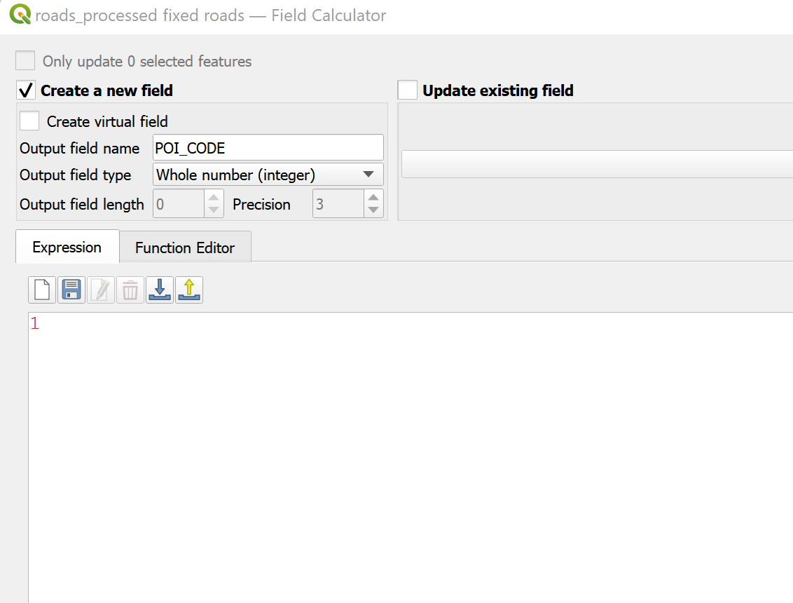
• Right click on the layer > Open Attribute Table. In the window that opens, select “Create Calculated Field”.

• In the window that opens, make sure ‘Create a New Field’ is selected. Enter “POI_CODE” into the field name and 1 into the box with the values. Then create the field by clicking on “Run”.

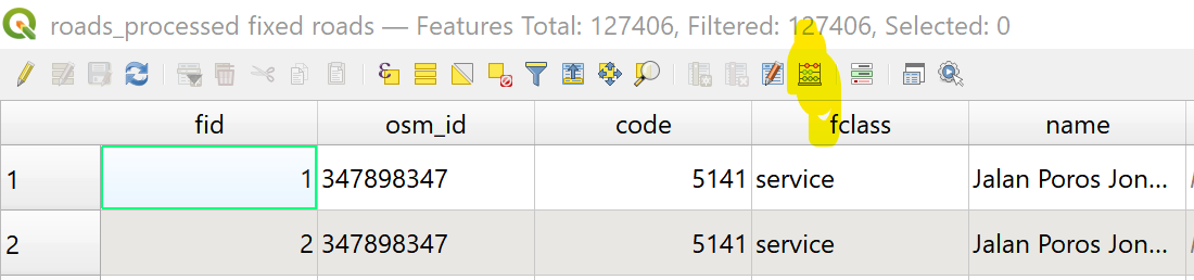
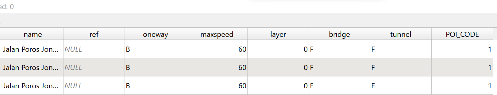
• To verify that it is created correctly in the attribute table there should be an additional column that is named “POI_CODE” with all values inside being 1.

Section 2.1. Preparing River Proximity and Road Proximity

• There is no extra processing needed for these layers.
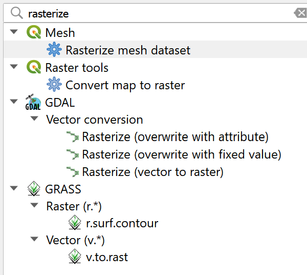
• Go to Processing Toolbox on the Right Hand Side of the page and select Rasterize.

* We use a 100x100m grid. In the window that opens, we set the field to burn-in to POI_CODE, the units to “Georeferenced Units”, and the height and width to 100, as seen below. The layer extent will follow the shape of the study area, with the layer “FinalShape”.

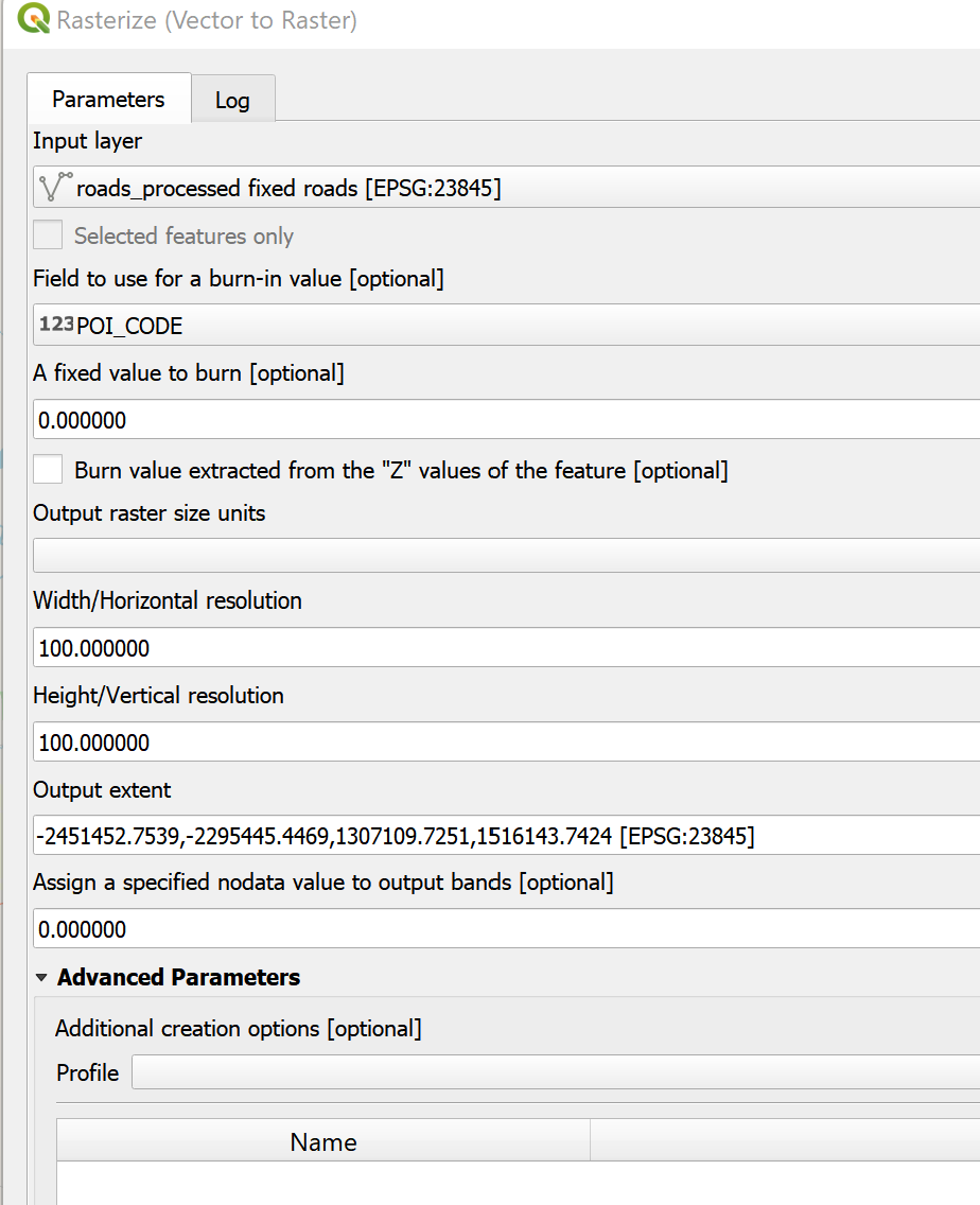
• When all is done, press “Run” and a rasterised layer should come up.

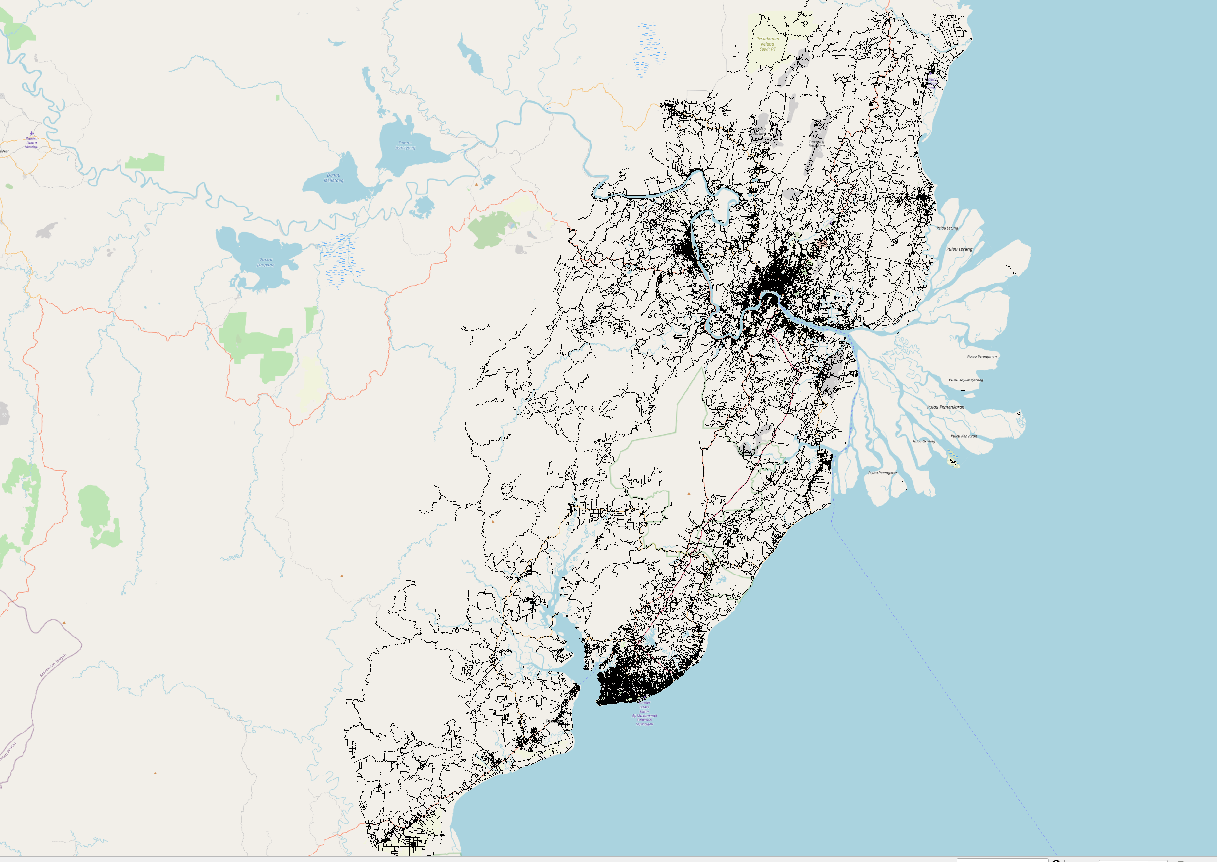
• Repeat this exercise for the layers for River and Seaport.

Section 2.2. Preparing Forest Layer

• This forest layer should have been prepared in the data preparation for Task 1, under the “Area” data format in “Clipping Layers”, including the filtering of appropriate areas for analyses.
• Repeat the steps in section 2.1.

Section 2.3. Preparing Distance from Airport

• Because the airport demand a buffer that is about 3km for noise abatement procedures, the nearest suitable area from the airport should be at least 3km proximity. Therefore, we would need to create a buffer around the airport before rasterising the entire buffer.
• To do this, go to Vector > Geoprocessing Tools > Create Buffer. In the window that appears, select the airport vector layer.
• In the resultant layer, ensure that the distance is set to 3000m, which would create a 3km buffer, and segments is set to 100, which would create a nice curved edge, instead of smaller values which woud result in a rectangle shaped buffer.

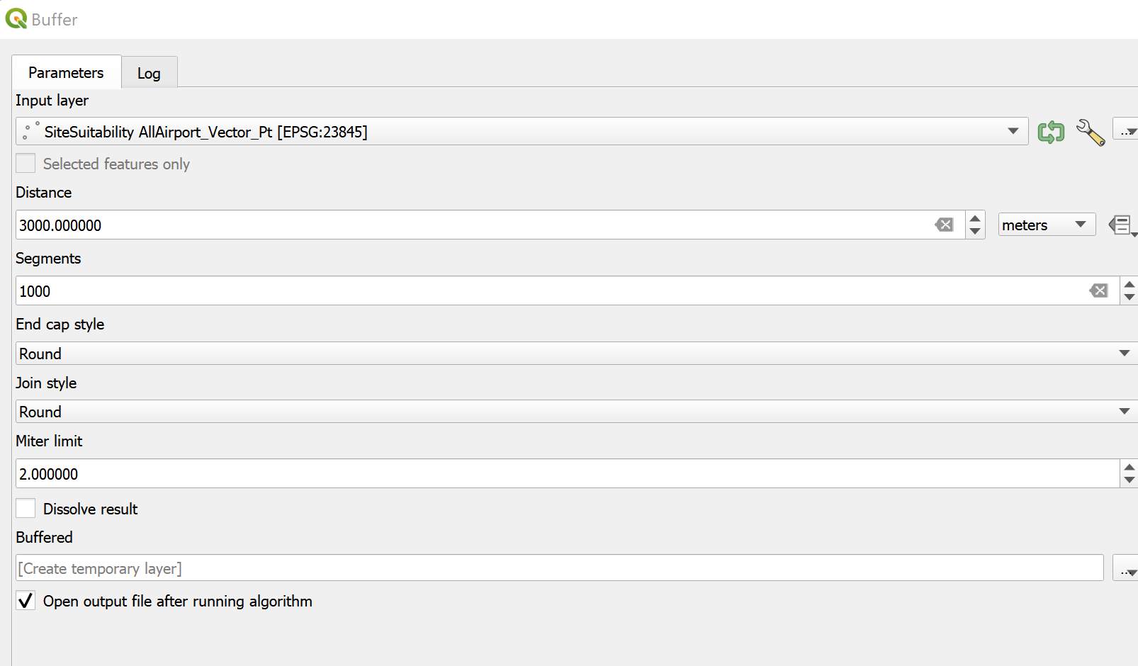
• After that, we click on “Run” to create a buffer. The result should look something like this.

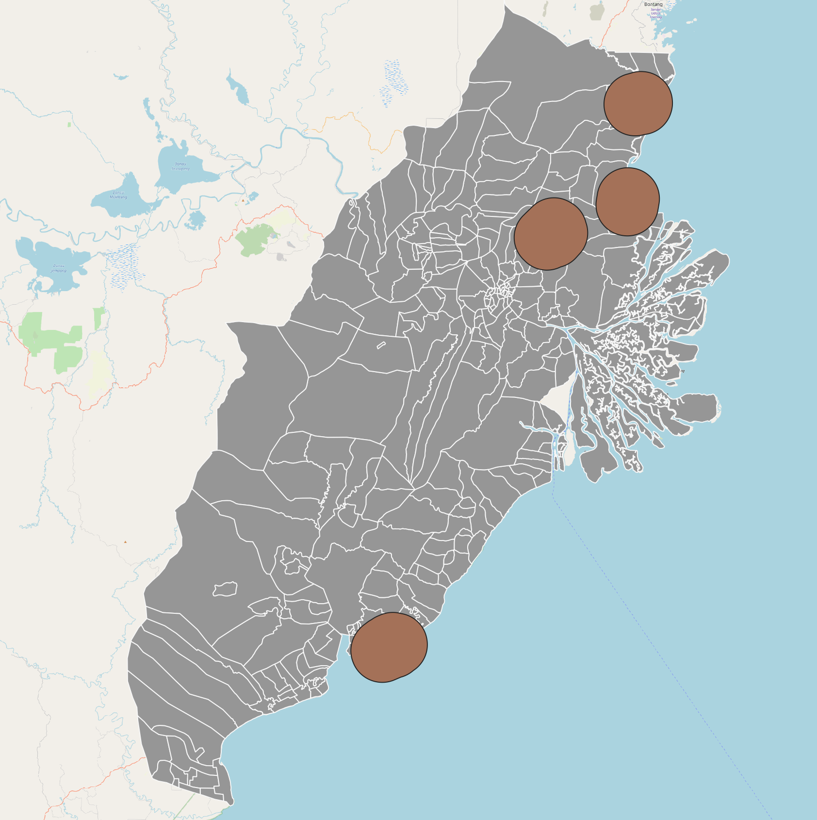
• Following that, we have to rasterise the layers. Now, we can continue with the steps as provided in section 2.1.

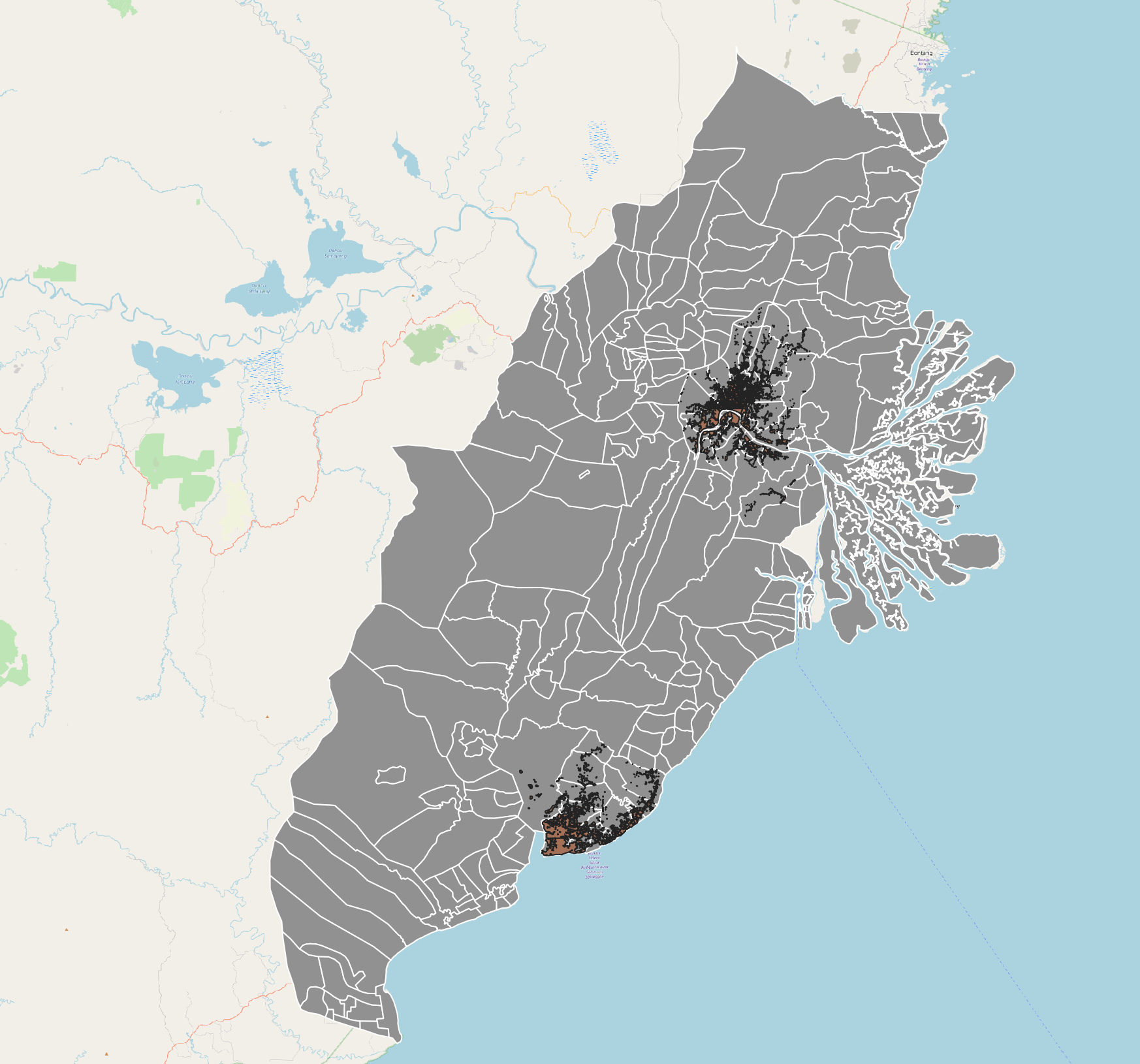
Section 2.4. Preparing Distance from Settlement

• This layer requires some clipping of the entire urban settlements layer, as has been prepared in task 1 under the “area type data”.

• We will need to clip the urban settlements with respect to the city boundaries of Kota Balikpapan and Kota Samarinda.

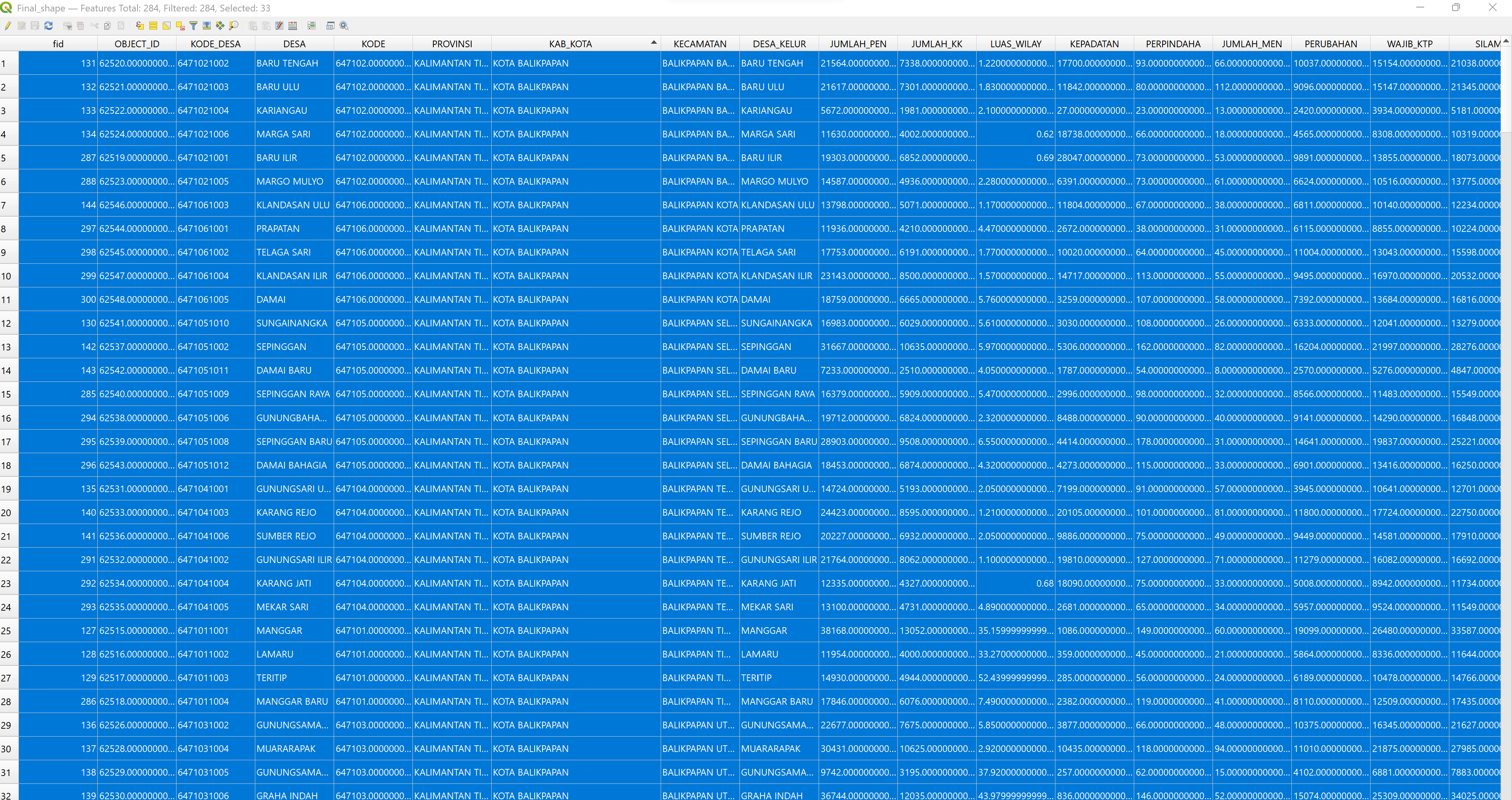
• We toggle the editing by clicking the pencil icon near the top of the window.

• Following that, we sort the table by “KAB_KOTA” by clicking on it, and then selecting all the rows with attribute KAB_KOTA = “KOTA BALIKPAPAN” or “KOTA_SAMARINDA”.

• We then exit the attribute table, go to the top panel and toggle editing by clicking on the pencil button on the top bars. Then we press CTRL+C to copy the features that we have selected.
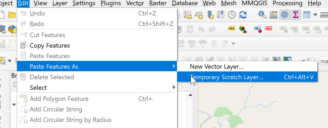
• We paste the features in a temporary layer by going to Edit > Paste > Temporary Scratch Layer.

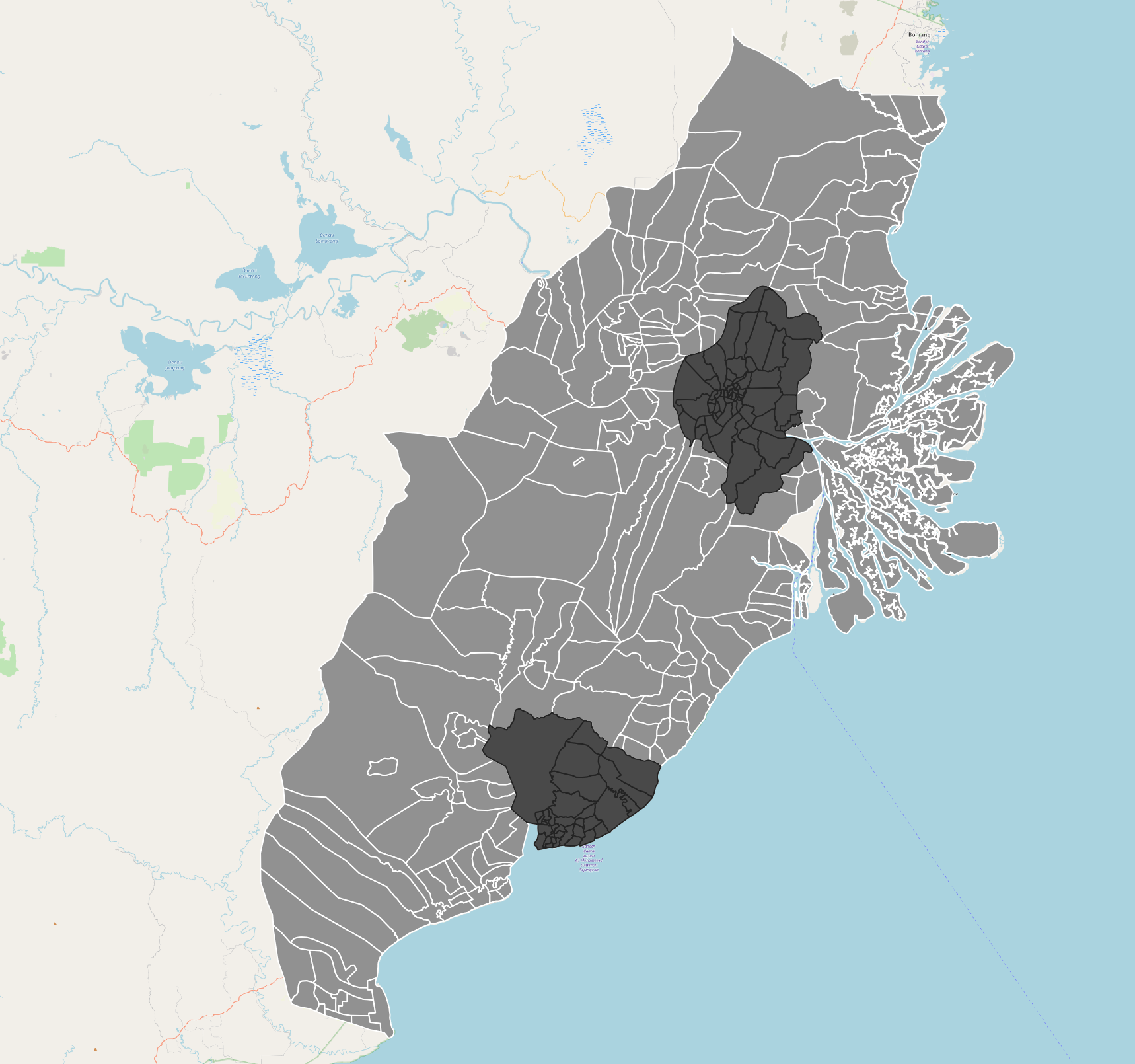
• We should see something like this, where the city limits are shaded differently because they are now on a temporary layer.

• Now we can proceed with the clipping.
• We now select the Urban Settlement layer.
• We then go to Vector > Geoprocessing > Clip and select the temporary layer with the city limits as the overlay layer, and the urban settlement layer as the input layer.

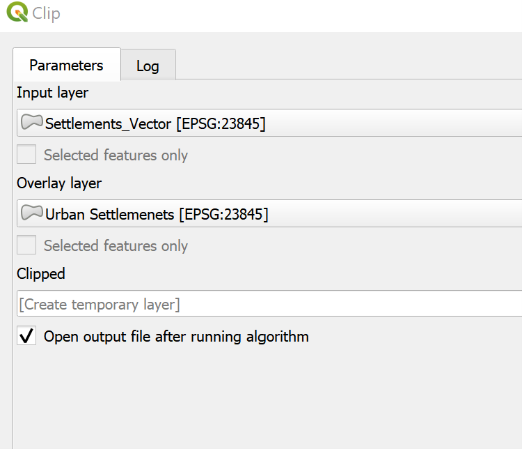
• We then click on “Run”. We should see that the urban settlement vector layer contains only those that are within the city limits.

• We can then proceed with following the steps from section 2.1, to rasterise the layer.